PyTorch 性能剖析(第三篇):注意力机制(Attention)全解析
文章背景与核心概要
本文是“PyTorch 性能剖析”系列教程的第三篇。在相继探讨了基础算术运算(第一篇)以及线性层与 MLP(第二篇)之后,本文将目光转向现代 Transformer 架构的核心组件:注意力机制(Attention)。
文章通过 PyTorch 性能剖析器(Profiler),详细对比了手写的朴素注意力机制与 PyTorch 原生 Scaled Dot Product Attention (SDPA) 及其多种底层后端(math、efficient、flash 和 cudnn)在 NVIDIA A100 GPU 上的实际表现。通过深入剖析剖析器追踪图(trace),我们揭示了隐藏的内存拷贝开销、张量核心(Tensor Core)的利用差异、显存带宽瓶颈,以及算子融合(Kernel Fusion)如何显著加速 Transformer 的工作负载。
Executive Summary
This article is the third installment in the Profiling in PyTorch series. Following our exploration of basic arithmetic operations (Part 1) and linear layers/MLPs (Part 2), this post tackles the fundamental architecture of modern transformers: Attention.
We analyze how different attention implementations appear under the PyTorch profiler, comparing a hand-written naive attention mechanism against PyTorch's native Scaled Dot Product Attention (SDPA) and its various backends (math, efficient, flash, and cudnn). By learning to read profiler traces, we uncover hidden memory copies, tensor core utilization differences, memory traffic bottlenecks, and how kernel fusion radically accelerates transformer workloads.
本文是《PyTorch 性能剖析》系列的第三篇文章。继第一篇探讨基础算术运算、第二篇探讨线性层与 MLP 之后,本文聚焦于现代 Transformer 的核心架构:注意力机制(Attention)。
我们分析了不同的注意力机制实现方式在 PyTorch 性能剖析器下的表现,对比了手写的朴素注意力机制与 PyTorch 原生的
缩放点积注意力 (SDPA)及其多种后端(math、efficient、flash和cudnn)。通过学习如何解读剖析器追踪图,我们揭示了隐藏的内存拷贝、张量核心利用率的差异、显存流量瓶颈,以及算子融合如何彻底加速 Transformer 工作负载。
Introduction to the Series
This series is designed to help you build the intuition required to read profiler traces and tables to drive targeted model optimizations: 1. Profiling in PyTorch (Part 1): A Beginner's Guide to torch.profiler 2. Profiling in PyTorch (Part 2): From nn.Linear to a Fused MLP 3. Profiling in PyTorch (Part 3): Attention is all you profile (current)
While attention is famous for its quadratic-time complexity, many clever optimizations exist to mitigate this bottleneck. Our goal here is to examine how each optimization strategy looks under the hood of an NVIDIA A100-SXM4-80GB GPU using the PyTorch profiler.
Note: The scripts for this blog post live in the repository:
04_a_naive_attention.py,04_b_inplace_ops_attention.py,04_c_sdpa_attention.py, and04_d_kernels_attention.py.系列简介
本系列旨在帮助读者建立阅读剖析器追踪图(Profiler Traces)和数据表的直觉,从而推动针对性的模型优化: 1. PyTorch 性能剖析(第一篇):torch.profiler 新手指南 2. PyTorch 性能剖析(第二篇):从 nn.Linear 到融合 MLP 3. PyTorch 性能剖析(第三篇):注意力机制全解析 (当前文章)
尽管注意力机制以其二次方的时间复杂度而闻名,但目前已有许多巧妙的优化方法来缓解这一瓶颈。我们此处的目是通过 PyTorch 剖析器,深入检视各种优化策略在
NVIDIA A100-SXM4-80GBGPU 底层的实际表现。注意: 本博客的脚本存放在仓库中:
04_a_naive_attention.py、04_b_inplace_ops_attention.py、04_c_sdpa_attention.py和04_d_kernels_attention.py。
Naive Attention
Attention processes Queries (\(q\)), Keys (\(k\)), and Values (\(v\)) through a sequential pipeline:
1. Compute attention scores: scores = matmul(q, k.T)
2. Scale scores: scores * scale
3. Apply a causal mask: scores.masked_fill(mask, "-inf")
4. Normalize with softmax: attn = softmax(scores)
5. Reweight values: matmul(attn, v)
Here is a naive implementation in PyTorch:
class NaiveCausalAttention(nn.Module):
    def __init__(self, head_dim):
        super().__init__()
        self.scale = 1.0 / math.sqrt(head_dim)

    def forward(self, q, k, v, mask):
        scores = torch.matmul(q, k.transpose(-2, -1))
        scores = scores * self.scale
        scores = scores.masked_fill(mask, float("-inf"))
        attn = torch.softmax(scores, dim=-1)
        out = torch.matmul(attn, v)
        return out
When profiling this implementation (uv run 04_a_naive_attention.py), we expect a series of distinct operations: matrix multiplications, scaling, masking, and softmax.
| Figure 1: The CPU lane highlighting discrete operations |
|---|
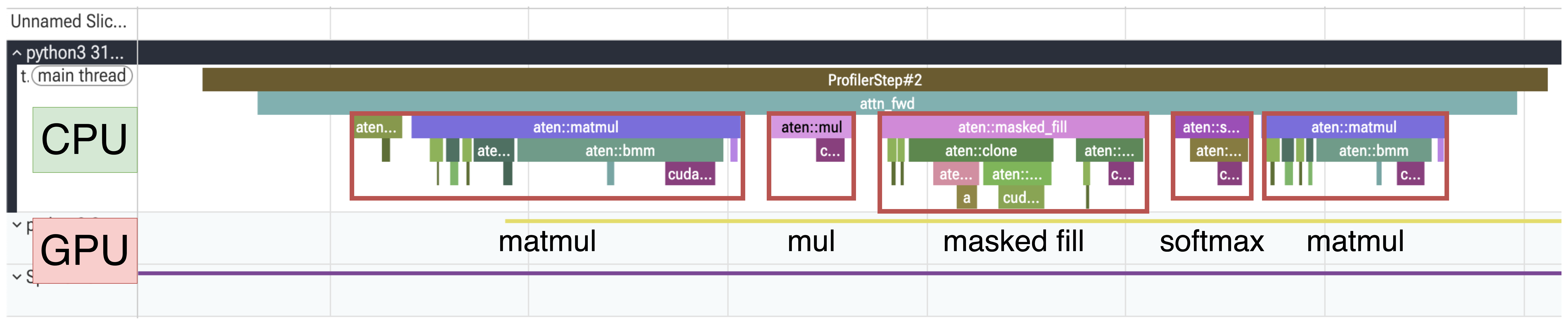 |
When unfolding the GPU lane, we can inspect the exact sequence of launched kernels:
| Figure 2: GPU and CPU lanes highlighting kernel collections |
|---|
 |
Zooming in on a single step reveals an unexpected guest: a Memory Copy (Memcpy) kernel.
| Figure 3: Zoomed-in GPU lane showing individual kernels |
|---|
 |
朴素注意力机制(Naive Attention)
注意力机制通过一个顺序流水线处理查询(\(q\))、键(\(k\))和值(\(v\)): 1. 计算注意力得分:
scores = matmul(q, k.T)2. 得分缩放:scores * scale3. 应用因果掩码:scores.masked_fill(mask, "-inf")4. 使用 softmax 进行归一化:attn = softmax(scores)5. 对值进行加权:matmul(attn, v)以下是 PyTorch 中的一个朴素实现:
class NaiveCausalAttention(nn.Module):
    def __init__(self, head_dim):
        super().__init__()
        self.scale = 1.0 / math.sqrt(head_dim)

    def forward(self, q, k, v, mask):
        scores = torch.matmul(q, k.transpose(-2, -1))
        scores = scores * self.scale
        scores = scores.masked_fill(mask, float("-inf"))
        attn = torch.softmax(scores, dim=-1)
        out = torch.matmul(attn, v)
        return out
在剖析此实现(
uv run 04_a_naive_attention.py)时,我们预期会看到一系列独立的连续操作:矩阵乘法、缩放、加掩码和 softmax。
图 1:高亮显示离散操作的 CPU 通道 展开 GPU 通道后,我们可以检查所启动的精确内核序列:
图 2:高亮显示内核集合的 GPU 与 CPU 通道 放大到单步执行时,会发现一个意料之外的访客:内存拷贝(
Memcpy)内核。
图 3:显示单个内核的放大 GPU 通道
Fixing the Memory Copy with In-Place Causal Masking
The out-of-place nature of standard masked_fill forces PyTorch to allocate a copy of the tensor, execute the fill, and return it. By switching to the in-place equivalent (masked_fill_), we eliminate this overhead:
# Before: scores = scores.masked_fill(mask, float("-inf"))
# After:
scores.masked_fill_(mask, float("-inf"))
| Type | CPU Stream Comparison |
|---|---|
| Figure 4: Naive Masking | |
| Figure 5: In-Place Masking |  |
Looking at the GPU lanes, the Memcpy kernel completely vanishes:
| Type | GPU Stream Comparison |
|---|---|
| Figure 6: Naive Masking | |
| Figure 7: In-Place Masking |  |
使用原地(In-Place)因果掩码消除内存拷贝
标准
masked_fill的非原地(out-of-place)特性迫使 PyTorch 分配张量的副本、执行填充并将其返回。通过切换到原地等效操作(masked_fill_),我们消除了这一开销:# 之前:scores = scores.masked_fill(mask, float("-inf")) # 之后: scores.masked_fill_(mask, float("-inf"))
类型 CPU 流对比 图 4: 朴素掩码 图 5: 原地掩码 观察 GPU 通道,
Memcpy内核完全消失了:
类型 GPU 流对比 图 6: 朴素掩码 图 7: 原地掩码
Scaled Dot Product Attention (SDPA)
PyTorch bundles the complete attention pipeline into a single optimized function:
from torch.nn import functional as F

F.scaled_dot_product_attention(q, k, v, is_causal=True)
SDPA dynamically dispatches to different backends depending on the hardware, inputs, and constraints. We can pin specific backends using the torch.nn.attention.sdpa_kernel context manager.
1. The Math Backend
Running uv run 04_c_sdpa_attention.py --backend math reveals a surprising result: the one-liner is roughly 3.7x slower than our naive in-place attention implementation.
| Metric | Naive In-Place | SDPA Math |
|---|---|---|
*_fwd CUDA time avg |
1.955 ms | 7.239 ms |
| Self CUDA time total | 7.194 ms | 27.279 ms |
While our naive implementation launches 5 kernels, the math backend launches 20 kernels per forward pass:
* Tensor Cores Left Vacant: Instead of utilizing high-performance Tensor Cores (e.g., s16816 instructions in bfloat16), it falls back to ordinary CUDA cores using sgemm (FP32), upcasting tensors and doubling data movement.
* Rebuilt Causal Masks: Passing is_causal=True causes the backend to materialize a fresh lower-triangular mask on every call via aten::ones, aten::tril, and aten::where.
* Safe Softmax: It executes _safe_softmax to handle fully masked rows and prevent NaN generation (0/0), introducing additional arithmetic overhead.
缩放点积注意力 (SDPA)
PyTorch 将完整的注意力流水线打包成一个单一的优化函数:
from torch.nn import functional as F

F.scaled_dot_product_attention(q, k, v, is_causal=True)
SDPA 根据硬件、输入和约束条件动态调度到不同的后端。我们可以使用
torch.nn.attention.sdpa_kernel上下文管理器来锁定特定的后端。1. 数学后端(Math Backend)
运行
uv run 04_c_sdpa_attention.py --backend math会揭示一个令人惊讶的结果:这行单行代码比我们的朴素原地注意力实现慢大约 3.7 倍。
指标 朴素原地实现 SDPA 数学后端 *_fwdCUDA 平均时间1.955 ms 7.239 ms 自定义 CUDA 总时间 7.194 ms 27.279 ms 我们的朴素实现启动了 5 个内核,而数学后端在每个前向传播中启动了 20 个内核: * Tensor Core 处于闲置状态: 它没有利用高性能 Tensor Core(例如 bfloat16 中的
s16816指令),而是回退到使用普通 CUDA 核心和sgemm(FP32),这会提升张量精度并使数据移动量翻倍。 * 重建因果掩码: 传入is_causal=True会导致后端在每次调用时通过aten::ones、aten::tril和aten::where重新生成一个新的下三角掩码。 * 安全 Softmax(Safe Softmax): 它执行_safe_softmax来处理全掩码行并防止产生NaN(0/0),从而引入了额外的算术开销。
2. The Efficient Backend (xFormers)
uv run 04_c_sdpa_attention.py --backend efficient
| Figure 14: Profiler trace for SDPA with efficient backend |
|---|
 |
The efficient backend (derived from Meta's xFormers) collapses the entire attention routine into a single fused kernel: fmha_cutlassF_bf16_aligned_64x64_rf_sm80. It operates directly in bf16 using Tensor Cores and keeps working sets in fast register memory (rf).
2. 高效后端(xFormers)
uv run 04_c_sdpa_attention.py --backend efficient
图 14:带有高效后端的 SDPA 剖析追踪图 高效后端(源自 Meta 的 xFormers)将整个注意力常规流程压缩为一个单一的融合内核:
fmha_cutlassF_bf16_aligned_64x64_rf_sm80。它直接在bf16中使用 Tensor Core 运行,并将工作集保留在快速寄存器内存(rf)中。
3. The Flash Backend (FlashAttention-2)
uv run 04_c_sdpa_attention.py --backend flash
| Figure 15: Flash backend trace |
|---|
 |
FlashAttention-2 (void pytorch_flash) solves the core bottleneck of attention: HBM (High Bandwidth Memory) traffic.
Traditional attention writes intermediate [seq, seq] score matrices (millions of elements) back and forth to global memory. FlashAttention processes keys and values in tiles, utilizing an online softmax trick to accumulate outputs incrementally without ever materializing the massive score matrix in global memory.
Understanding Occupancy: Profilers may report low occupancy (e.g., 13%) for FlashAttention kernels. This occurs because Flash allocates significant shared memory and heavy register usage per block (e.g., 255 registers per thread). This low occupancy is intentional—it trades thread-level concurrency to keep data in on-chip SRAM and prevent expensive global memory round-trips.
3. Flash 后端(FlashAttention-2)
uv run 04_c_sdpa_attention.py --backend flash
图 15:Flash 后端追踪图 FlashAttention-2(
void pytorch_flash)解决了注意力的核心瓶颈:HBM(高带宽内存)流量。传统的注意力机制会在全局内存中来回读写中间的
[seq, seq]得分矩阵(包含数百万个元素)。而 FlashAttention 以分块(tiles)的形式处理键和值,利用在线 Softmax(online softmax)技巧来增量累加输出,而无需在全局内存中实际生成巨大的得分矩阵。理解占用率(Occupancy): 剖析器可能会报告 FlashAttention 内核的占用率较低(例如 13%)。这是因为 Flash 在每个块中分配了大量的共享内存并高强度使用寄存器(例如每个线程 255 个寄存器)。这种低占用率是有意为之的——它牺牲了线程级的并发性,从而将数据保留在片上 SRAM 中,并防止了昂贵的全局内存往返。
4. The cuDNN Backend
uv run 04_c_sdpa_attention.py --backend cudnn
| Figure 18: cuDNN backend trace |
|---|
 |
NVIDIA's cuDNN backend dynamically generates and tunes a custom attention kernel specifically tailored to the runtime shape and problem profile:
- No Transposes: Unlike flash or efficient backends which require metadata reshapes, cuDNN consumes native
[B, H, S, D]layouts directly. - Driver-Level Launch: It launches via
cuLaunchKernelExrather than the standard runtime APIcudaLaunchKernel. - CPU Overhead: While the GPU kernel executes efficiently, the CPU time is significantly higher (approx. 214 µs vs 138 µs for flash) due to the runtime plan-selection and "knob" tuning performed on every call.
4. cuDNN 后端
uv run 04_c_sdpa_attention.py --backend cudnn
图 18:cuDNN 后端追踪图 NVIDIA 的 cuDNN 后端会根据运行时的形状和问题特征,动态生成并调优专用的自定义注意力内核:
- 无需转置: 与需要元数据重塑(reshapes)的 flash 或 efficient 后端不同,cuDNN 直接消费原生的
[B, H, S, D]布局。- 驱动层启动: 它通过
cuLaunchKernelEx启动,而不是标准的运行时 APIcudaLaunchKernel。- CPU 开销: 尽管 GPU 内核执行效率很高,但由于每次调用时都会执行运行时方案选择和“参数(knob)”调优,因此 CPU 时间明显更高(约为 214 µs,而 flash 为 138 µs)。
Summary of Attention Variants
| Variant | What We Changed | Kernels / Forward | Key Takeaway |
|---|---|---|---|
| Naive Attention | Built using primitive PyTorch ops | 6 | Out-of-place masked_fill introduces a hidden Memcpy kernel. |
| Naive In-Place | masked_fill \(\rightarrow\) masked_fill_ |
5 | In-place operation eliminates the Memcpy overhead entirely. |
| SDPA Math | Pinned to SDPBackend.MATH |
20 | Reference implementation; uses FP32 on CUDA cores, making it correct but \(\sim\)3.7x slower. |
| SDPA Efficient | xFormers-backed implementation | 1 | Fused fmha_cutlassF kernel running natively in bf16 on Tensor Cores. |
| SDPA Flash | FlashAttention-2 (pytorch_flash) |
1 | Eliminates global memory traffic via tiling; fastest overall performance. |
| SDPA cuDNN | cuDNN generated backend | 1 | Dynamically tuned kernel with zero transposes, though plan generation increases CPU overhead. |
注意力变体总结
变体 更改内容 单次前向内核数 核心要点 朴素注意力 使用 PyTorch 原语构建 6 非原地的 masked_fill引入了隐藏的Memcpy内核。朴素原地实现 masked_fill\(\rightarrow\)masked_fill_5 原地操作完全消除了 Memcpy开销。SDPA 数学后端 锁定到 SDPBackend.MATH20 参考实现;在 CUDA 核心上使用 FP32,正确但慢约 3.7 倍。 SDPA 高效后端 基于 xFormers 的实现 1 融合的 fmha_cutlassF内核,在 Tensor Core 上以bf16原生运行。SDPA Flash FlashAttention-2 ( pytorch_flash)1 通过分块消除全局内存流量;整体性能最快。 SDPA cuDNN cuDNN 生成的后端 1 动态调优的内核,无需转置,但方案生成增加了 CPU 开销。
Conclusion
The golden rule of profiling covered throughout this series is simple: Guess first, then look.
By stating your expectations before opening a trace, unexpected behaviors—such as hidden memory copies, fallback to CUDA cores, or heavy CPU dispatch costs—transform from confusing anomalies into valuable insights. Profiling is not an esoteric black art; it is simply the practice of asking "Why is that happening?" until the bottleneck is revealed.
Now open up a trace, formulate your hypothesis, and start optimizing! 🤗
结论
本系列贯穿始终的剖析黄金法则很简单:先猜测,后查看。
通过在打开追踪图之前陈述您的预期,那些意料之外的行为——例如隐藏的内存拷贝、回退到 CUDA 核心或沉重的 CPU 调度成本——就会从令人困惑的异常转变为有价值的洞察。性能剖析并非深奥的黑魔法;它只是一种不断追问“为什么会这样?”直到揭示瓶颈的实践。
现在,打开一个追踪图,提出您的假设,开始优化吧!🤗